Excel Conditional Formatting Tutorial: Highlight Data Automatically

Conditional formatting in Excel automatically changes cell colors, adds data bars, or displays icons based on rules you define — making patterns, outliers, and trends visible at a glance without manual formatting. Once set up, the formatting updates automatically when data changes. For more Excel skills, see our intermediate Excel tutorial.

Key Takeaways

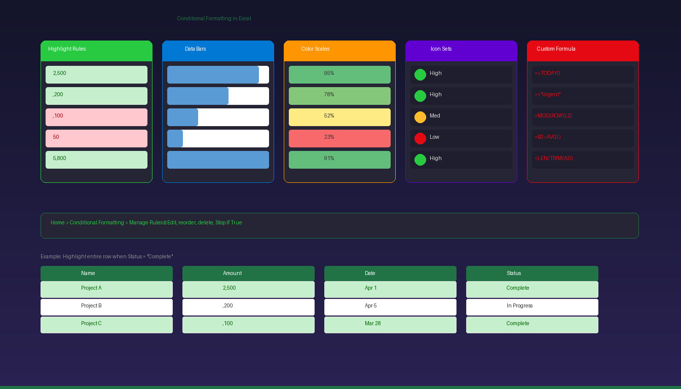
• Access conditional formatting via Home > Conditional Formatting — choose from Highlight Cell Rules, Top/Bottom Rules, Data Bars, Color Scales, or Icon Sets.
• Custom formula rules (=formula) let you create complex conditions like highlighting entire rows based on multiple criteria.
• Use Manage Rules (Home > Conditional Formatting > Manage Rules) to edit, reorder, or delete existing rules — rules higher in the list take priority.

How Do I Apply Basic Highlight Rules?

Select a range, go to Home > Conditional Formatting > Highlight Cell Rules, and choose a condition — cells matching the criteria are automatically highlighted with the color you select.

Built-In Highlight Rules

1. Select the data range.
2. Go to Home > Conditional Formatting > Highlight Cell Rules.
3. Choose a rule:

Rule	What It Highlights	Example
Greater Than	Values above a threshold	Sales > $10,000
Less Than	Values below a threshold	Inventory < 50
Between	Values within a range	Scores between 70-89
Equal To	Exact matches	Status = “Overdue”
Text That Contains	Cells containing specific text	Name contains “Smith”
A Date Occurring	Dates in a time period	Due dates this week
Duplicate Values	Repeated or unique values	Find duplicate email addresses

1. Set the threshold value and formatting (fill color, text color).
2. Click OK.

Top/Bottom Rules

Go to Conditional Formatting > Top/Bottom Rules:

Rule	What It Highlights
Top 10 Items	Highest N values
Top 10%	Top percentage of values
Bottom 10 Items	Lowest N values
Bottom 10%	Bottom percentage of values
Above Average	Values above the range average
Below Average	Values below the range average

These are ideal for quickly identifying best and worst performers in sales data, grades, or KPIs.

How Do I Use Data Bars, Color Scales, and Icon Sets?

These visual formats show relative values within cells — data bars act as mini bar charts, color scales create heatmaps, and icon sets add status indicators.

Data Bars

1. Select the data range.
2. Go to Conditional Formatting > Data Bars.
3. Choose a Gradient Fill or Solid Fill color.

Each cell displays a horizontal bar proportional to its value — longer bars = larger values. Data bars work best for numerical columns where you want quick visual comparison.

Color Scales

1. Select the range > Conditional Formatting > Color Scales.
2. Choose a 2-color or 3-color scale (e.g., Green-Yellow-Red).

Scale Type	Best For
Green-Red	Performance metrics (green = good, red = bad)
Blue-White-Red	Temperature or deviation from average
Green-Yellow-Red	Traffic light status visualization
White-Blue	Intensity/density heatmaps

Color scales create instant heatmap visualizations — ideal for large data tables where individual values are hard to compare manually.

Icon Sets

1. Select the range > Conditional Formatting > Icon Sets.
2. Choose from arrows, flags, traffic lights, stars, or bars.

Icons appear inside each cell based on value thresholds. Default thresholds split values into equal segments, but you can customize them through Manage Rules.

According to Microsoft Support, icon sets work best with 3-5 categories — they lose effectiveness with too many data points at similar values.

How Do I Create Custom Formula Rules?

Use a formula rule to apply conditional formatting based on complex logic — the formula must return TRUE or FALSE, and you can reference other cells to format entire rows based on a single column’s value.

Create a Formula Rule

1. Select the range to format.
2. Go to Conditional Formatting > New Rule.
3. Select Use a formula to determine which cells to format.
4. Enter a formula that returns TRUE/FALSE.
5. Click Format to set colors, borders, or font.
6. Click OK.

Common Formula Examples

Goal	Formula	What It Does
Highlight overdue	=$D2<TODAY()	Formats if date in column D is past
Highlight entire row	=$E2="Urgent"	Formats row if column E says “Urgent”
Alternate row shading	=MOD(ROW(),2)=0	Formats every other row
Highlight weekends	=WEEKDAY($A2,2)>5	Formats Saturday/Sunday dates
Above column average	=B2>AVERAGE($B:$B)	Formats values above the column average
Non-blank cells	=LEN(TRIM($A2))>0	Formats only cells with content

Key: Mixed References

When formatting entire rows based on one column, use $ before the column letter (e.g., $E2) to lock the column while letting the row adjust. Without the $, the formula shifts incorrectly when applied across multiple columns.

How Do I Manage and Edit Existing Rules?

Go to Home > Conditional Formatting > Manage Rules to view, edit, reorder, or delete all conditional formatting rules on the current selection or entire worksheet.

Open the Rules Manager

1. Go to Home > Conditional Formatting > Manage Rules.
2. Change Show formatting rules for to:
3. Current Selection — rules on selected cells only
4. This Worksheet — all rules on the sheet

Rules Manager Actions

Action	How	Effect
Edit rule	Select rule > Edit Rule	Change conditions or formatting
Delete rule	Select rule > Delete Rule	Remove the formatting rule
Reorder	Use Up/Down arrows	Higher rules take priority
Stop If True	Check the checkbox	Prevents lower rules from applying
Change range	Edit “Applies to” field	Expand or shrink the formatted range

Rule Priority

When multiple rules apply to the same cells, the rule highest in the list takes priority. Use “Stop If True” to prevent conflicting rules from overriding each other. For example: if Rule 1 highlights overdue items in red and Rule 2 highlights all items above $1,000 in green, an overdue item above $1,000 would be green (Rule 2 wins) unless Rule 1 has “Stop If True” checked.

How Do I Format Entire Rows Based on a Cell Value?

Select the entire data range (all columns), create a New Rule with a formula, and use a mixed reference ($column) to lock the condition column while formatting all columns in the row.

Step-by-Step

Example: Highlight the entire row when Status (column E) = “Complete”

1. Select the entire data range: A2:F100.
2. Go to Conditional Formatting > New Rule > Use a formula.
3. Enter: =$E2="Complete"
4. Click Format > Fill > choose green.
5. Click OK twice.

Every row where column E contains “Complete” is highlighted green across all columns A through F. The $E locks to column E while 2 adjusts for each row.

What Are Conditional Formatting Best Practices?

Use conditional formatting purposefully — too many rules create visual clutter and slow down large workbooks.

Do	Avoid
Use 2-3 rules per range	More than 5 rules on one range
Use consistent colors	Different color meanings per sheet
Green = good, Red = bad	Reversed color conventions
Apply to Excel Tables	Formatting static ranges (miss new data)
Use formulas for complex logic	Nesting multiple simple rules
Name your ranges	Applying rules to entire columns (A:A) — slows workbook
Document your rules	Leaving undocumented rules for others to decode

For building dashboards with conditional formatting, see our Excel dashboard tutorial. For more Excel data analysis, see our Excel formulas tutorial. If you need Excel with full conditional formatting, Microsoft Office 2024 Professional Plus ($199.99) includes the complete Excel desktop application.

Frequently Asked Questions

---