How to Create and Use Lookup Tables in Excel

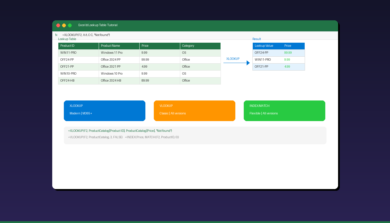
A lookup table in Excel is a structured reference sheet that stores data you frequently need — like product prices, employee IDs, or tax rates — so you can pull values automatically using formulas instead of typing them manually. The three main lookup methods are XLOOKUP (modern), VLOOKUP (classic), and INDEX/MATCH (flexible). If you are new to Excel, start with our Excel tutorial for beginners first.

Key Takeaways

• A lookup table is a structured data range with a unique identifier in the first column and related values in adjacent columns — convert it to an Excel Table (Ctrl+T) for automatic expansion.
• XLOOKUP is the recommended lookup function for Microsoft 365 and Excel 2021+ — it replaces VLOOKUP with simpler syntax, left-right lookups, and built-in error handling.
• VLOOKUP still works in all Excel versions but only looks right, breaks when columns are inserted, and requires a column index number.

How Do I Create a Lookup Table in Excel?

Set up a separate sheet or range with a unique identifier column and related data columns, then convert it to an Excel Table for automatic expansion and easier formula references.

Step 1: Structure Your Lookup Data

Create a range with clear headers and one unique value per row:

Product ID	Product Name	Price	Category
WIN11-PRO	Windows 11 Pro	$99.99	Operating System
OFF24-PP	Office 2024 Professional Plus	$199.99	Office Suite
OFF21-PP	Office 2021 Professional Plus	$64.99	Office Suite
WIN10-PRO	Windows 10 Pro	$59.99	Operating System

Step 2: Convert to an Excel Table

1. Click anywhere in the data range.
2. Press Ctrl+T.
3. Confirm the range and check My table has headers.
4. Click OK.
5. In the Table Design tab, give the table a name (e.g., “ProductCatalog”).

Excel Tables automatically expand when you add new rows, so your lookup formulas always include the latest data without manual range adjustments.

Step 3: Use Named Ranges (Optional)

For even cleaner formulas, name individual columns:

1. Select the Product ID column (without header).
2. Click in the Name Box (left of formula bar).
3. Type ProductIDs and press Enter.
4. Repeat for other columns (ProductNames, Prices).

How Do I Use XLOOKUP With a Lookup Table?

XLOOKUP searches a column for a value and returns the corresponding value from any other column — use it with the syntax =XLOOKUP(lookup_value, lookup_array, return_array).

Basic XLOOKUP

To look up a product price by Product ID:

=XLOOKUP(A2, ProductCatalog[Product ID], ProductCatalog[Price])

This searches for the value in A2 within the Product ID column and returns the matching price. If no match is found, XLOOKUP returns #N/A by default.

XLOOKUP With Error Handling

=XLOOKUP(A2, ProductCatalog[Product ID], ProductCatalog[Price], "Not found")

The fourth argument replaces #N/A with “Not found” — no need for IFERROR() wrappers.

XLOOKUP Returning Multiple Columns

=XLOOKUP(A2, ProductCatalog[Product ID], ProductCatalog[Product Name]:ProductCatalog[Category])

This returns Product Name, Price, and Category in one formula — the result spills across multiple cells.

XLOOKUP Key Features

Feature	Description
Default search	Exact match (no need to specify)
Direction	Searches any direction (left, right)
If not found	Built-in error handling argument
Multiple returns	Returns multiple columns in one formula
Approximate match	Optional: -1 (exact or next smaller), 1 (exact or next larger)
Search mode	First-to-last (default), last-to-first, binary search

According to Microsoft Support, XLOOKUP is available in Microsoft 365 and Excel 2021 or later. It is not available in Excel 2019 or earlier.

How Do I Use VLOOKUP With a Lookup Table?

VLOOKUP searches the first column of a range and returns a value from a specified column number — use the syntax =VLOOKUP(lookup_value, table_array, col_index_num, FALSE).

Basic VLOOKUP

=VLOOKUP(A2, ProductCatalog, 3, FALSE)

This searches for A2 in the first column of ProductCatalog and returns the value from column 3 (Price). FALSE specifies an exact match.

VLOOKUP Limitations

Limitation	Impact	Workaround
Right-only lookup	Cannot return values from columns to the left	Use XLOOKUP or INDEX/MATCH
Column index breaks	Inserting/deleting columns changes the index number	Use MATCH for dynamic index
Single return	Returns one value per formula	Use separate formulas per column
No built-in error handling	Returns #N/A on no match	Wrap with IFERROR()
First match only	Returns first match in unsorted data	Sort data or use XLOOKUP

For a detailed VLOOKUP guide with more examples, see our Excel VLOOKUP tutorial.

How Do I Use INDEX/MATCH With a Lookup Table?

INDEX/MATCH combines two functions — MATCH finds the row position, INDEX returns the value at that position — making it more flexible than VLOOKUP and compatible with all Excel versions.

Basic INDEX/MATCH

=INDEX(ProductCatalog[Price], MATCH(A2, ProductCatalog[Product ID], 0))

• MATCH(A2, ProductCatalog[Product ID], 0) — finds which row A2 appears in (0 = exact match)
• INDEX(ProductCatalog[Price], ...) — returns the Price from that row

Left Lookup With INDEX/MATCH

Unlike VLOOKUP, INDEX/MATCH can look up values to the left:

=INDEX(ProductCatalog[Product ID], MATCH("Office 2024 Professional Plus", ProductCatalog[Product Name], 0))

This finds the Product ID for a given Product Name — impossible with VLOOKUP since Product ID is to the left of Product Name.

Two-Way Lookup

Look up a value based on both row and column criteria:

=INDEX(DataRange, MATCH(row_value, RowHeaders, 0), MATCH(col_value, ColHeaders, 0))

This is useful for cross-reference tables like tax rate lookups where you need to match both income bracket and filing status.

Which Lookup Method Should I Use?

Use XLOOKUP for new workbooks on Microsoft 365 or Excel 2021+, INDEX/MATCH for backward compatibility or complex lookups, and VLOOKUP only for maintaining existing workbooks.

Feature	XLOOKUP	VLOOKUP	INDEX/MATCH
Availability	M365, Excel 2021+	All versions	All versions
Syntax simplicity	Simple (3 args)	Moderate (4 args)	Complex (nested)
Look left	Yes	No	Yes
Column insert safe	Yes	No (index breaks)	Yes
Error handling	Built-in argument	Needs IFERROR()	Needs IFERROR()
Multiple returns	Yes (spill)	No	No
Approximate match	Optional argument	TRUE/FALSE	1/0/-1
Performance	Fast	Fast	Fast
Best for	New workbooks (M365)	Legacy compatibility	Complex/flexible lookups

Decision Flow

1. Using Microsoft 365 or Excel 2021+? → Use XLOOKUP
2. Need backward compatibility with Excel 2019 or earlier? → Use INDEX/MATCH
3. Maintaining an existing workbook with VLOOKUP? → Keep VLOOKUP (no need to rewrite)
4. Need a left lookup or dynamic column reference? → Use XLOOKUP or INDEX/MATCH

How Do I Handle Common Lookup Errors?

The most common lookup errors are #N/A (no match found), #REF (invalid reference), and #VALUE (wrong data type) — each has specific causes and fixes.

Error	Cause	Fix
#N/A	Lookup value not found in table	Check spelling, extra spaces (use TRIM), data type mismatch
#REF!	Column index exceeds table width (VLOOKUP)	Reduce col_index_num or use XLOOKUP
#VALUE!	Wrong argument type	Verify lookup_value matches the data type in lookup column
#SPILL!	XLOOKUP spill range blocked	Clear cells in the spill area
Wrong result	Approximate match returning wrong value	Use FALSE (VLOOKUP) or 0 (MATCH) for exact match
Extra spaces	Hidden spaces cause mismatch	Use =TRIM() on lookup value and/or lookup column

Wrap With Error Handling

VLOOKUP/INDEX-MATCH:

=IFERROR(VLOOKUP(A2, ProductCatalog, 3, FALSE), "Not found")

XLOOKUP (built-in):

=XLOOKUP(A2, ProductCatalog[Product ID], ProductCatalog[Price], "Not found")

For more Excel formulas and functions, see our Excel pivot table tutorial. If you need Excel with XLOOKUP support, Microsoft Office 2024 Professional Plus ($199.99) includes Excel 2024 with all modern functions including XLOOKUP, LAMBDA, and dynamic arrays.

Frequently Asked Questions

---